¶ personally thank all those programmers who build lots of cool and useful applications on internet and many of them deliver it free of cost, but they lack in theoretical computer science background. For that reason i came up with this idea and turned on my P.C and started typing.The idea behind theoretical computer science is Algorithm Analysis, trust me you are all going to love this because this going help you to deal with programming pragmatically since you have the art but not the background.
So I am done with my babbling and lets make it quick and simple..
Understanding Algorithm Analysis leads you dealing with girls more pragmatically , may be this was the whole point for me to learn Algorithm Analysis .
Overview:
- Time Complexity
- Comparing Algorithms
- The Classes P
- The Class NP
- The Class NP-Complete
- The Class NPI
Time Complexity
As you know girls don’t come easy and each have different keys to unlock, same are the algorithms(considered as problems).
Problems are solvable or unsolvable
Solvable : Hurrah!! She accepted my proposal. 😆
Unsolvable : She takes too much time. 😳
Therefore in programming life too we face the same problem of algorithms, which cannot be solved in reasonable time and are considered as practically unsolvable. Another thing which we should consider in the storage space.So it brings to this conclusion :
- Time
- Space
Now that you know about the type of girls that exists , its time to tell you some thing or two about them :
- Speed of the processor
- Quality of the compiler
- Size of the input
- And most importantly the Measure of performance of an algorithm.
Trust me if are willing to follow such rules in understanding the complexity of any girl i’ll bet you are in the right direction,Oh boy!!
Now finally the most important part of all , how do you actually find the complexity? have any idea..
Very disappointing, since you don’t have the answer let me say it-
1. Experimental Study –
It is just like going and asking every girl more like a try-error policy
Let me show an example :
<br />import java.io.*;<br /><br />class for1<br /><br />{<br /><br />public static void main(String args[]) throws Exception<br /><br />{int N,Sum;<br /><br />N=1000;//N value can be changed.<br /><br />Sum=0;<br /><br />long start=System.currentTimeMillis(); // this going to give you the start time<br /><br />int i,j;<br /><br />for(i=0;i<N;i++)<br /><br />for(j=0;j<i;j++)<br /><br />Sum++;<br /><br />long end=System.currentTimeMillis();// this going to give you the end time<br /><br />long time=end-start; // this way u get ur total time in millis<br /><br />System.out.println('The start time is :'+start);<br /><br />System.out.println('The endtime is :'+end);<br /><br />System.out.println('The time taken is :'+time);<br /><br />}<br /><br />}<br />
Run it and plot the result and you will be getting a graph like this..
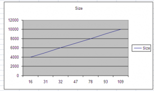
In this way you can study each and every algorithm performance.
2.Theoretical Analysis –
Its more of a trained way of understanding a girl but in my personal opinion I prefer the Experimental one though it beats me a lot.
Time complexity of algorithms are expressed using the O-notation.
The complexity of a function f(n) is O(g(n)) if |f(n)| ≤ c×|g(n)| for all n>0 and some constant c.
Let f and g be functions on n, then:
f(n) = O(g(n)) means that “f is of the order of g”, that is, “f grows at the same
rate of g or slower”.
f(n) = W(g(n)) means that “f grows faster than g”
f(n) = Q(g(n)) means that “f and g grow at the same rate”.
An algorithm is said to perform in polynomial time iff its time complexity function
is given by O(nk) for some k ³ 0.
That is, an algorithm A is polynomial time if timeA(n) <= f(n) and f is a polynomial,
i.e. f has the form: a1nk + a2nk-1 +…+ am
Now this might look a bit confusing ,but read it twice to swallow it permanently.It works!
Lets check out some examples:
Example 1:
3x2 + 2x + 2 = O(x2) because
3x2 + 2x + 2 <= 5×2 for x > 1
3×2 + 2x + 2 <=7×2 for x > 0
We say that f » g (f is equivalent to g) if f = O(g) and g = O(f).
Example 2:
x2 = O(3x2 + 2x + 2) because
x2 <= 3x2 + 2x + 2 for x >= 0
Then we could say that 3x2 + 2x + 2 » x2.
An algorithm is said to perform in exponential time if its complexity function is not bounded by a polynomial but instead is given by O(cn) for some c > 1.
Comparing Algorithms
Let two algorithms A and B for solving a problem ∏ and let timeA and timeB be
the time complexities of algorithms A and B respectively.
Algorithm A is said to have the same complexity as algorithm B in solving ∏ if:
timeA » timeB
Algorithm A is said to be better than algorithm B in solving ∏ if:
timeA is O(timeB) but timeB is not O(timeA)
Example:
Let algorithms A, B with time complexities as shown below. How do
these two algorithm compare? timeA(n) ={ 1,000,000 for n ≤1,000,000; n for n > 1,000,000} timeB(n) ={n2 for n > 1,000,000 ; n for n ≤ 1,000,000} timeA(n) = O(timeB) but timeB(n) ≠ O(timeA) which means that algorithm A is better than algorithm B (although for practical purposes this may not be the case).
A problem ∏ is said to be tractable if there is a known polynomial time algorithm
to solve it. A problem ∏ is said to be intractable if it is solvable but there is no
known polynomial time algorithm to solve it.
Having a problem ∏ and an algorithm to solve it that is not polynomial time, then
the option is to search for a better algorithm, i.e. a polynomial time one.
Enough!! 😳 she takes too much time, lets move on, Sad but True. This reminds me of someone 😳
Class P
Class P is known as PTIME or DTIME ,is one of the most fundamental complexity classes.Remember these classes were introduced to make things easier not to make them more complicated. It contains all decision problems which can be solved by a deterministic Turing machine using a polynomial amount of computation time(or polynomial time).So does that make things easier ? At least you have a class to deal with.Don’t ask what is a Turing machine,because there’s a whole lot of things to say.. anyway in short it is a device that manipulates symbols on a strip of tape according to a table of rules.So it can be adapted to simulate any logic or algorithm.And most importantly it explains the nature of the CPU of any computer.
Note:
All the algorithms which falls under Class P are said to be efficiently solvable or tractable.
Given the decision TSP: for a set of n cities C={c1,c2,…,cn} and a distance
between each pair of cities ci and cj given by dij € Z+. Is there a tour of all cities,
starting and ending in city c1 and visiting each city exactly once, such that the
total distance traveled ≤ b?
The number of possible tours is (n-1)!
A deterministic machine would be able to explore only one tour at a time so it would take exponential time to solve the decision TSP.
There is no known deterministic machine that can solve the decision TSP in polynomial time.
Let be M a deterministic Turing machine and input x € S*.The time complexity timeM of a deterministic Turing machine M is given by timeM(n) = max{m | there is an x € Sn such that the computation of M on input x is of length m}
If timeM(n) is O(nk) for some k >= 0 then M is said to take polynomial time.
The Turing machine M is an algorithm is if halts for all inputs and then timeM(n)is defined for all n.Then, the class P is defined as the class of problems which can be solved by
polynomial time deterministic algorithms. Problems in P can be solved ‘quickly’.
P = { L | there is a polynomial time deterministic TM which accepts L}
Every language in P is a recursive language.
Class NP
In this case the decision TSP , a non-deterministic machine (with unlimited parallelism) would be able to solve the decision TSP in polynomial time.Let be NDTM a non-deterministic Turing machine and input x € S*.Then there is at least one computation sequence (possibly more) by which NDM accepts x.
The time taken by NDTM to accept x is given by the length of the shortest of the computation sequences by which NDTM accepts x.
The time complexity timeNDM of a non-deterministic Turing machine NDTM is
given by:
timeNDM(n) =
{
1 if no inputs on length n are
accepted by NDTM;
min{m | there is an x € Sn such otherwise
that the time taken by NDTM to
accept x is m };
}
NDTM is polynomial time iff timeNDM(n) is O(nK) for some k > 0.Then, the class NP is defined as the class of problems which can be solved by
polynomial time non-deterministic algorithms. Problems in NP can be verified
‘quickly’.
NP = { L | there is a polynomial time non-deterministic TM which accepts L}
It should be clear that P subset of NP.
It is widely believed that P ≠NP but this has not been formally proven.
NP-Complete problems arise in many domains like: boolean logic; graphs, sets
and partitions; sequencing, scheduling, allocation; automata and language
theory; network design; compilers, program optimization; hardware
design/optimization; number theory, algebra.
Class NP-Complete
Then, within the class NP there are easy problems, those in P, and much
harder problems called NP-complete problems.
Intuitively, the class NP-complete are the hardest problems in NP as defined by
Cook’s theorem.
More formally, problem ∏ is NP-complete if ∏ € NP and for any ∏’ € NP ∏’ ∞ ∏.
Assume two problems ∏1, ∏2 and an algorithm A to solve ∏2. If each instance of
∏1 can be easily (in polynomial time) transformed into some instance of ∏2 then
we could use algorithm A to solve∏1.
Class NPI
Accepting that P ≠ NP does not mean necessarily that P U NP-complete = NP.
Some problems might not be in P neither in NP-complete.
It has been shown that if P = NP then NPI = NP – (P U NP-complete).
However, the vast majority of practical problems are in P or in NP-complete.
Example:
It is a conjecture that the decision problems: Graph Isomorphism and
Composite Number are both in NPI.
Graph isomorphism:
given two graphs G1 and G2, is G1 isomorphic to G2?
For the special case of G1,G2 being planar, the problem is solved in polynomial
time.
But no polynomial time algorithm has been found to solve the general case. And
no one has been able to prove that Graph Isomorphism is NP-complete.
Composite Number:
given a positive integer k, are there integer m,n > 1 such
that k = m×n?
If any polynomial time algorithm can be designed to test primality then the
problem would be in P but such an algorithm has not been found.
However, there is a polynomial time algorithm for solving the Composite Number
problem when k is not a prime number.

Pingback: trast.lekud.com